Stochastic gradient descent is an algorithm that tries to find the minimum of a function expressed as a sum of component functions. It does so by choosing a component function at random then following its gradient.
Sum functions
Suppose is expressed as the mean of component functions :
The gradient
The gradient of at is a vector directed along the steepest ascent at .
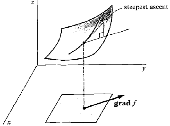
We can try to find the minimum of by taking iterative steps in the direction of . This is what the gradient descent algorithm do.
Sometimes, computing the gradient of is too computationally expensive. Stochastic gradient descent reduces the computational cost by using the gradient of one component function instead.
Stochastic gradient descent algorithm
The stochastic gradient descent algorithm aims at finding the minimum of by taking successive steps directed along , where at each step is chosen at random.
def stochastic_gradient_descent(f, x_0, max_steps, step_size):
    """
    f is a list such that f[n-1]
    is the n-th component function
    """
    x = x_0
    for step in range(max_steps):
        # Choose the component function at random
        n = random.randint(0, len(f)-1)
        # Update step
        x = x - step_size * gradient(of=f[n], at=x)
    return x
Comparison with gradient descent
The update rule for gradient descent at step t is:
While the update rule for stochastic gradient descent is:
| n is random |
Is it really faster than gradient descent?
For iterations, and training examples, gradient descent computes gradients while stochastic gradient descent computes only gradients. When , this yields a good optimization.
In practice SGD is worth a shot when we have a very large number of training examples. In machine learning, it often happens that we have hundreds of thousands, or millions of training examples (i.e. ) and that SGD still converges after only a few hundreds of iterations (i.e. ).
Why it works
This algorithm works because is an unbiased estimate of that is much simpler to compute.
Computational cost
The gradient of a sum is the sum of the gradients, so:
Which explains why is computationaly cheaper than .
Correctness
Furthermore, is an unbiased estimate for , indeed:
Where is the expectation taken over dthe distribution of (which is chosen randomly, remember).
Mini-batch SGD
There is a variant of stochastic gradient descent called mini-batch, where instead of using only one component function, several components functions are used. These component functions are chosen at random at each step.
In this version, instead of simply choosing one index at random, a subset is chosen at random. The update step of the algorithm is the same where is replaced by .
Comparison with SGD
The update rule for SGD at step t is:
| n is random |
While the update rule for mini-batch SGD at step t is:
| B is random |
The mini-batch algorithm
def minibatch_SGD(f, x_0, max_steps, step_size):
    """
    f is a list such that f[n-1]
    is the n-th component function
    """
    x = x_0
    for step in range(max_steps):
        # Choose B=[a;b] at random
        a = random.randint(0, len(f)-1)
        b = random.randint(a, len(f)-1)
        # Compute the sum of gradients
        sigma = sum([gradient(of=f[n], at=x) for n in range(a, b+1)])
        # Update step
        x = x - step_size * 1/(b-a+1) * sigma
    return x