The effect of L2-regularization

When fitting a model to some training dataset, we want to avoid overfitting. A common method to do so is to use regularization. In this article, we discuss the impact of L2-regularization on the estimated parameters of a linear model.

What is L2-regularization

L2-regularization adds a regularization term to the loss function. The goal is to prevent overfiting by penalizing large parameters in favor of smaller parameters. Let $\sets$ be some dataset and $\vw$ the vector of parameters:

$$\l_\text{reg}(\sets, \vw) = \underbrace{\l(\sets, \vw)}_\text{loss} + \underbrace{\lambda\normtwo{\vw}^2}_\text{regularizer}$$

Where $\lambda$ is an hyperparameter that controls how important the regularization

The effect of the hyperparameter

Increasing the $\lambda$ hyperparameter moves the optimal of $\l_\text{reg}$ closer to $0$, and away from the optimal for the unregularized loss $\l$.

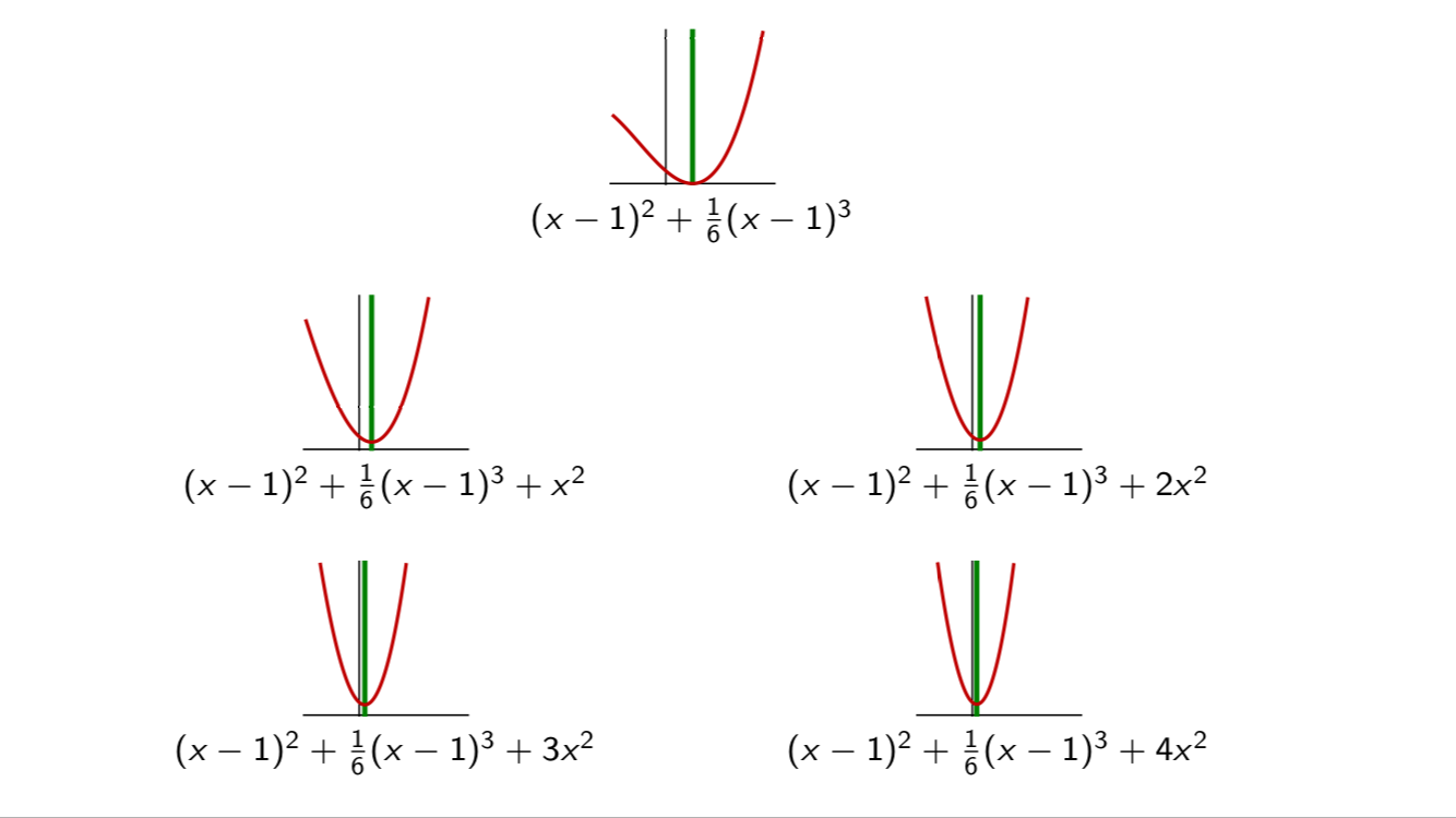
This can be visualized using one feature $\sx$ and a dataset made of one sample $(\sx, \sy)$. Take (for instance) the following loss:

$$\l(\sx, \{\sx\}) = (x - 1)^2 + \frac{1}{6}(x - 1)^3$$

The regularization term is:

$$\lambda\normtwo{\sx}^2 = \lambda\sx^2$$

On the graph below, we plotted this loss function (first graph) and several variant of the corresponding $\l_\text{reg}$ for different values of $\lambda = 0, 1, 2, 3, 4$. As the value of $\lambda$ increases, the loss curve is translated towards $0$.

This can be vizualized in 2D, where we see that the optimum of the regularized loss approaches $\vec{0}$ more and more when $\lambda$ increases. However, there is another way to conceptualize the regularization, which we will present next.

Regularization seen as constrained optimization

To understand how L2-regularization impacts the parameters, we will use an example in $\realvset{2}$.

Let’s note $\beta = (\beta_1, \beta_2)$ the vector of parameters.

Our estimate is:

$$\hat{\beta} = \argmin_{\beta} \l(\sets, \beta) + \lambda\normtwo{\beta}^2$$

Which is equivalent to a constrained optimization problem:

	minimize: $\l(\sets, \beta)$
	subject to: $\normtwo{\beta}^2 \leq \ss^2$

This formulation is easier to interpret: the selected vector of parameters $\hat{\beta}$ is the vector that minimzes the loss, among all vector inside the ball of radius $\ss$.

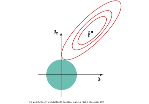
This is illustrated on the picture below. The red contour lines are the contour lines of the loss function $\l$. The unregularized optimal $\hat{\beta}$ is indicated by a black dot at the location of the minimum of $\l$. The ball of radius $\ss$ is drawn in blue. The solution to the constrained optimization is the intersection of the contour lines and the ball.

Effect on the individual parameters

What is the effect of the regularization on the individual parameters $\beta_1$ and $\beta_2$ ?

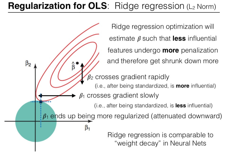
Regularized optimization will estimate $\beta$ such that less influential features undergo more penalization and therefore get shrunk down more.

On the plot above, $\beta_2$ crosses the gradient more rapidly that $\beta_1$ (we can see this as the contour lines are less separated along the $\beta_2$ axis than along the $\beta_1$ axis). When both $\beta_1$ and $\beta_2$ are standardized, this means that $\beta_2$ is more influential than $\beta_1$.

As a result, $\beta_1$ is more penalized by the L2-constraint than $\beta_2$.

This phenomenon explains why we should normalize the features before using regularization. More details on this in what follows.

Effect when approaching 0

Since the gradient of $\normtwo{\cdot}$ vanishes around $0$, the optimal will never move there if it was not already there. In other words: the parameters $\beta_\si$ are pushed towards $0$, but they are never set to $0$.

Another regularization method, the L1 regularization has a different behavior: since the gradient around $0$ do not vanish, the parameters $\beta_\si$ are pushed towards $0$ and may attain it and remain there. is.

Important remark about normalization

The regularizer term $\normtwo{\vw}^2$ treats each component the same way:

$$\normtwo{\vw}^2 = \sum_{\si = 1}^{\sd} \sw_{\si}^2$$

Therefore it is important to unify the scale of each feature vector $\vf_\si$. Indeed, suppose that the optimal solution is $\hat{\vw}$ for some design matrix $\mx$ where:

$$\mx = \begin{pmatrix} \uparrow & & \uparrow \\ \vf_1, & \dotsc, & \vf_\sd \\ \downarrow & & \downarrow \end{pmatrix}$$

The estimate $\hat{\vy}$ is:

$$\hat{\vy} = \mx\hat{\vw} = \sum_{\si = 1}^{\sd} \sw_{\si}\vf_{\si}$$

If we rescale one column of the design matrix, say $\vf^{r}_{0} = \epsilon\vf_{0}$, then we don’t bring new information and the estimate $\hat{\vy}$ should not change. The parameter $\sw^{r}_{0}$ is inversely rescaled:

$$\hat{\vy} = \mx\hat{\vw} = \mx^{r}\hat{\vw}^{r}$$

And:

$$\sw_0\vf_0 = \sw^{r}_0\vf^{r}_0 = \frac{\sw_0}{\epsilon}(\epsilon\vf_0)$$

But the parameters $\sw_0$ and $\sw^{r}_0 = \epsilon^{-1}\sw_0$ will be penalized with the same strength by the L2 regularization.

Therefore, to avoid mistaking influential parameters with non-influential ones because of scaling factors within the feature vector, we must normalize the features.

By norming the columns of $\mx$, we put them on the same scale. Consequently, differences in the magnitudes of the components of $\vw$ are directly related to the wiggliness of the regression function $\mx\vw$, which is loosely speaking what the regularization tries to control.

TL;DR: before using regularization, transform your feature vectors into unit vectors.