In this article, we define underfitting and overfitting and show some nice ways to vizualize them on polynomial regressions.
In short
Underfitting and overfitting describe the ability of a machine-learning model to make good predictions on datasets it wasn’t trained on.
Underfitting happens when:
- The model is too rigid to learn the true relationship in the data.
- Both test error and train error are large.
- The error is dominated by the bias error.
Overfitting happens when:
- The model is not rigid enough and mistakes noise for signal.
- The train error is low but the test error is large.
- The error is dominated by the variance error.
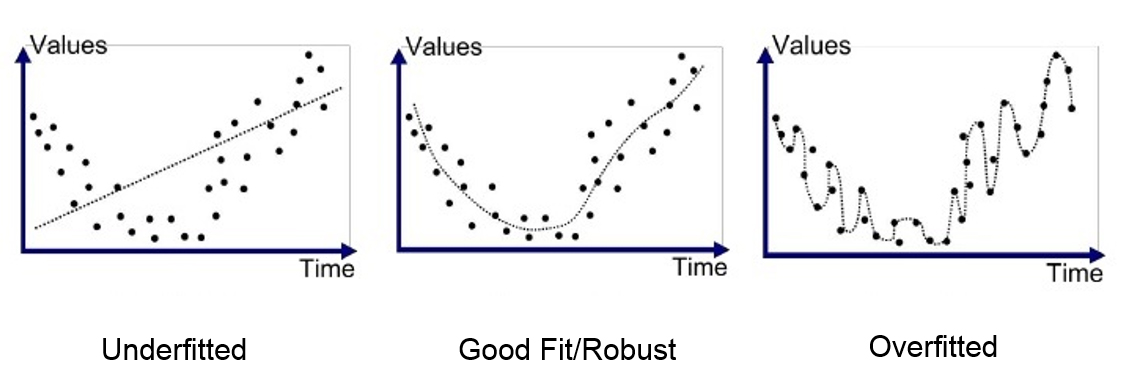
- The left hand side graph shows the underfitting scenario. We can see that the model is so rigid that is doesn’t fit the general shape of the data. This is called the bias of the model.
- The graph in the middle displays a good fit. The model fits the general shape of the data but does not wiggle too much between data points. This is the good bias-variance equilibrium.
- The right hand side graph shows the overfitting scenario. The model wiggles too much. And the general shape of the data is obfuscated by this high variance.
The signal and the noise
Let be a random vector. Given a deterministic function , we say that the random variable is a signal.
Let a gaussian noise with mean. The random variable is our signal polluted by the noise:
The train dataset, is made of independent observations of :
This means that for each observation , we have:
Where:
- is a realization of , whose value is known, and:
- is a realization of whose value is unknown.
Learning the signal
The goal of machine-learning is to learn the signal function from the inputs generated by and the outputs generated by . This task is made complex because of the unknown noise observations .
To do so, we suppose a model for the function and minimize the error between the observed outputs and the predictions .
While our end goal is to approximate , we can only do so by comparing our predictions with . Overfitting happens when our model “learns” the specifics of the noise realizations in the train dataset.
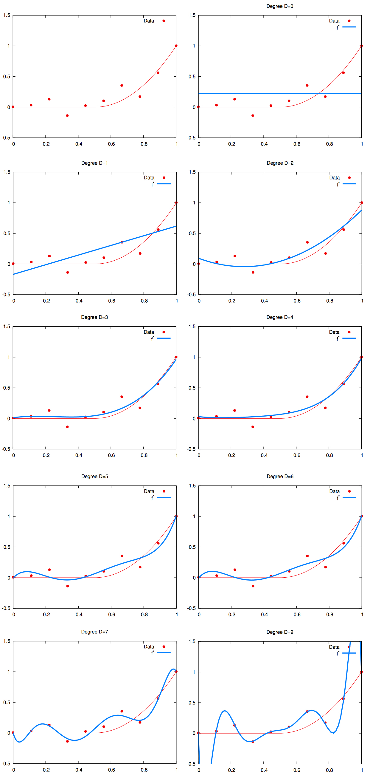
To illustrate overfitting, we will use polynomial regression. As the degree of the fitted polynomial increases, the model has more freedom to fit complex signals. But also more freedom to fit the unwanted noise.
This is illustrated on the picture below, where:
- the red curve is the real signal ;
- the red points are observed values for this signal, polluted by the random noise ;
- the blue curve is the regression line learned by a polynomial regression.
High variance
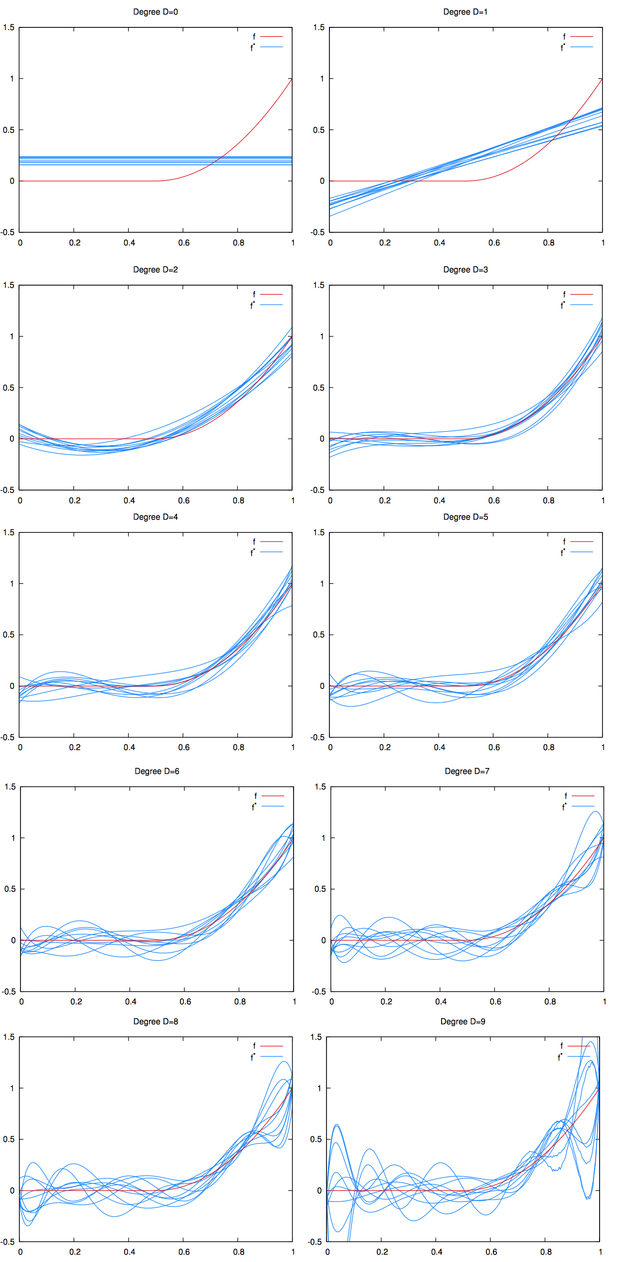
To better visualize the implications of overfitting on the regression curve, we can generate multiple train datasets, each with the same signal curve (in red), but with different random values for the noise . For instance:
and:
where and are different values for the noise, drawn from the same distribution.
Let’s generate a lot of train datasets like those.
If we fit a polynomial regression to each train dataset thus generated and we graph all the regression lines (in blue) on the same plot, we can visualize the high variance induced by overfitting. See picture below.
The Bias-Variance Tradeoff
Since we used a gaussian noise with mean, taking the mean of the regression curves should yield the signal. Indeed, as the number of train sets used increases, the mean of the noise observations converges to :
Hence:
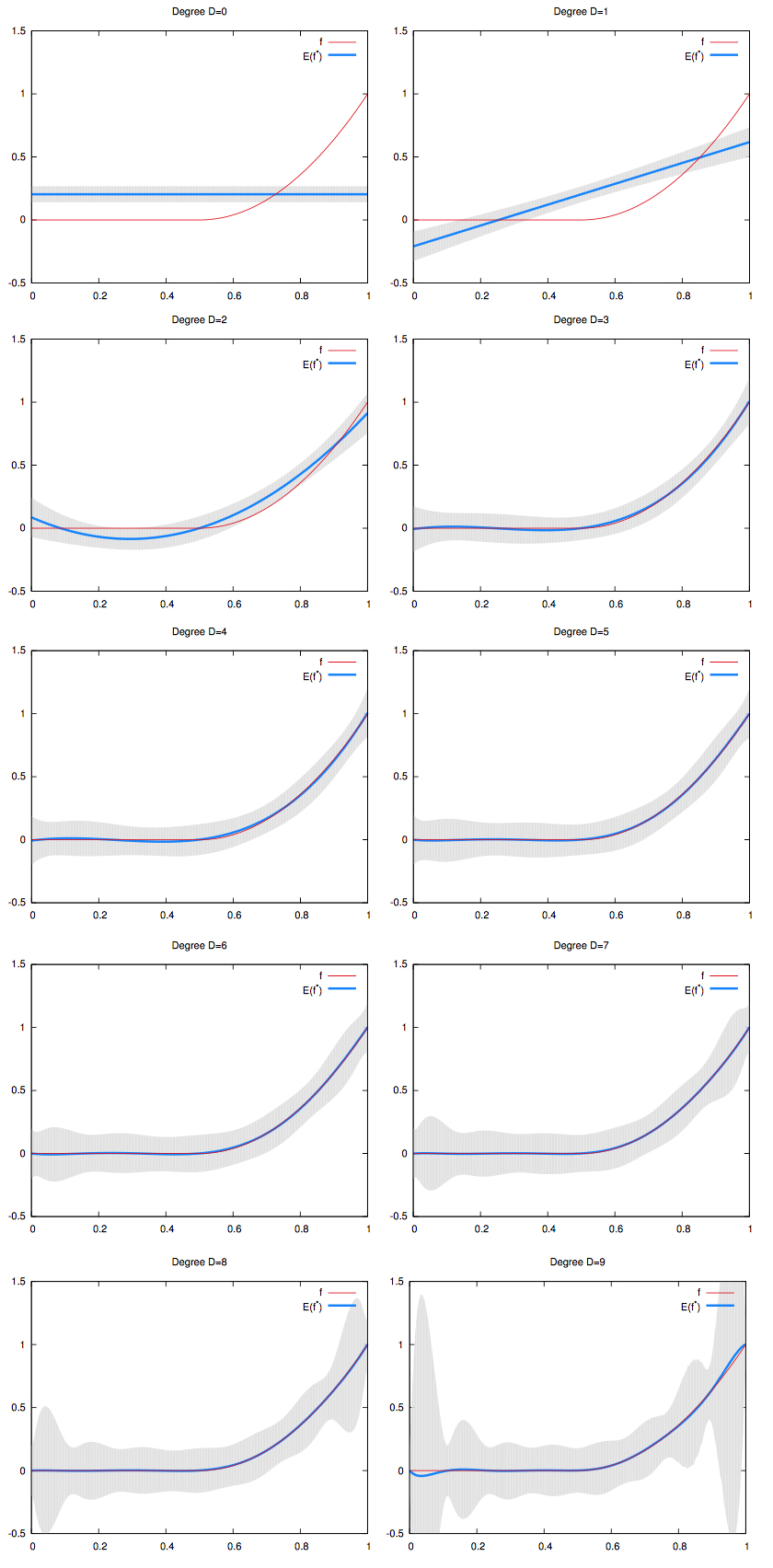
On the picture below, we graphed the mean of the regression curves in blue. The gray shape around it is the spread of all the regression curves.
- We can see that for low degree polynomials, the blue curve does not fit the red curve. We say that they have high bias. But the gray shape has small width. We say they have low variance.
- On the other hand, for high degree polynomials, the blue curve perfectly match the red curve. We say they have low bias. But the gray shape has large width. We say they have high variance.