We’ve just fitted OLS to our trainset. How to assess whether it was a good model to use? We will answer this question from the point of view of machine-learning and statistics.
Recall from our article about the difference between statistics and machine-learning that those fields asses their models differently. Machine-learning relies on the large size of modern datasets while statistics relies on theory.
So, how to we assess an OLS regression?
Machine-learning
In machine learning, we measure a model’s performance using the loss function. The fit is assessed by the training error:
While the generalization error is assessed by computing the loss on the testset :
To be meaningful, these measures require enough data.
As for preprocessing, rely on automated methods such as forward-selection or backward-elimination. But as we will see in the next section, the statistician’s approach provides usefull graohs that can guide and speed up this process.
Statistics
In statistics, we rely on statistical theory to produce ways to check if our model is adapted to the data at hand.
As discussed in our article about the theory underlying an OLS regression, the regression is asymptotically optimal when the output vector is normally distributed and the center of its distribution is a linear function of the input vectors:
Here is the output vector and the design matrix. is a vector of parameters.
We can rewrite this hypothesis using an error vector whose components are normally distributed: :
The strategy is to find implications of these assumptions that we can check graphically.
Checking for linearity
Under the assumption of linearity, the residual vector should be in the kernel of the design matrix . Hence the two following plots:
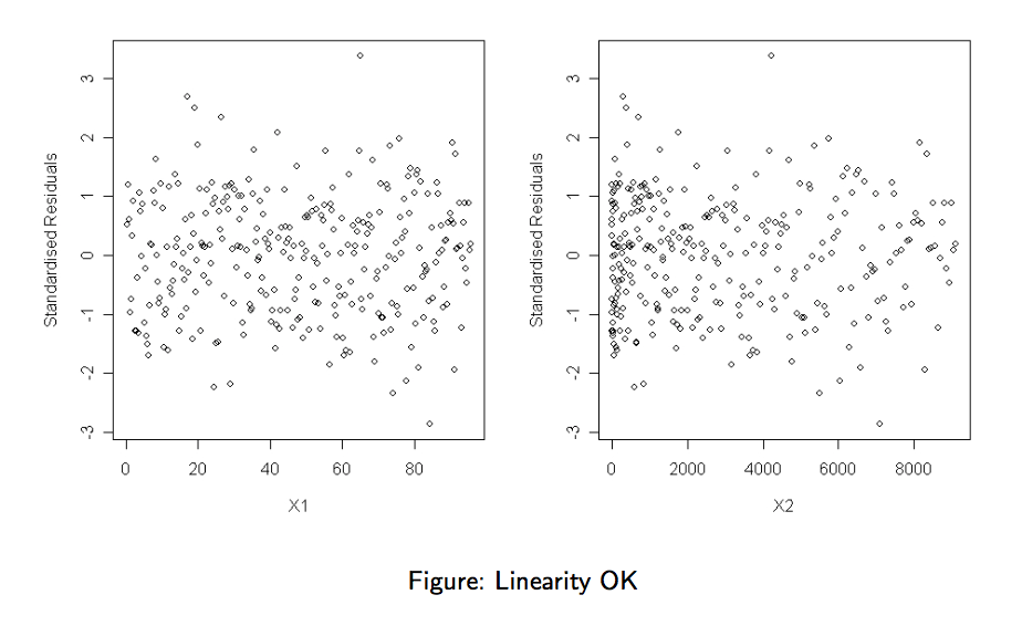
- Plot standardised residual against each feature (column of ). No systematic pattern should appear in these plots. A systematic pattern would suggest that we need to add a transformation of the current feature as an additional column.
In the plot below, no systematic pattern appears:
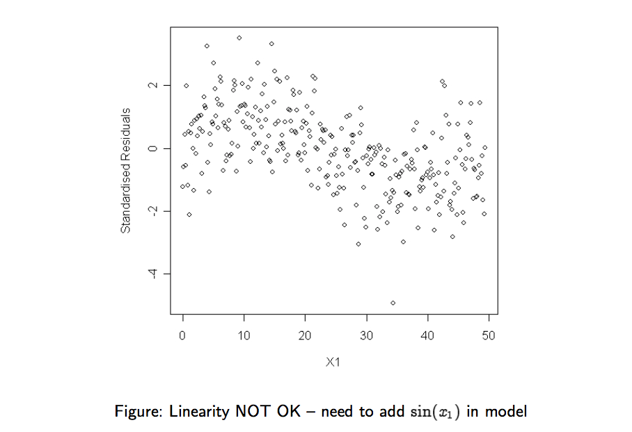
While on the plot below, we recognize a sinus pattern:
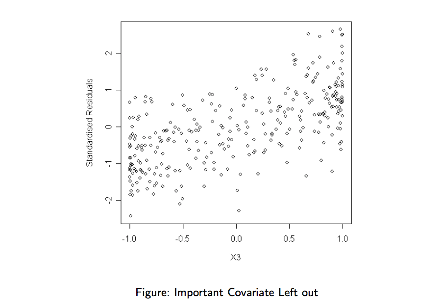
- Plot standardised residual against each feature that we left out of the model. No systematic pattern should appear in these plots. A Systematic pattern suggests that we have left out a feature that should have been included.
This is what the plot of a feature that should have been included looks like:
Checking for homoskedasticity
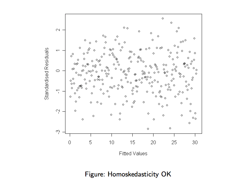
- Plot the standardised residuals against the estimates . A random scatter should appear, with approximately constant spread of the values of for the different values of . “Trumpet” of “bulging” effects indicate that the noise components are not i.i.d. (they have different variance).
This is what such plot should look like:
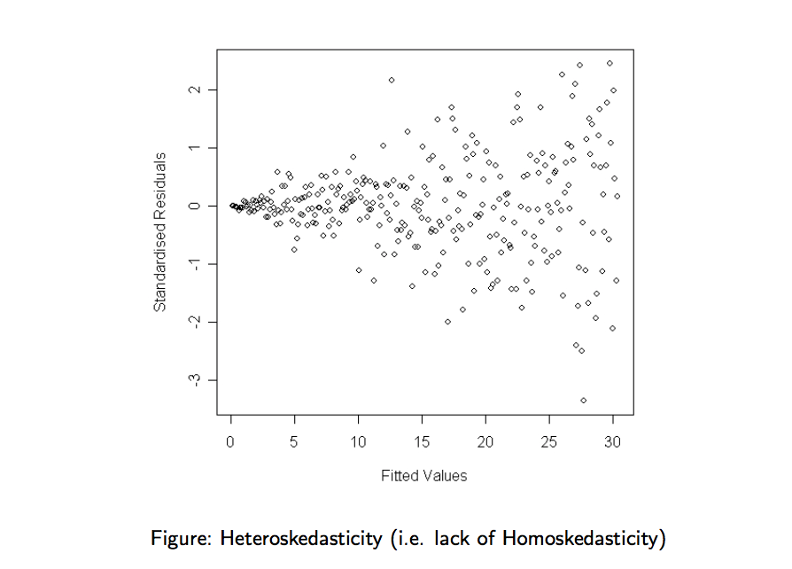
On the plot below, the noise components have different variance. Model assumptions not validated.
Checking for normality
We can compare the distribution of the standardised residual agains a normal distribution. This can be done by comparing theoretical quantiles with empirical ones.
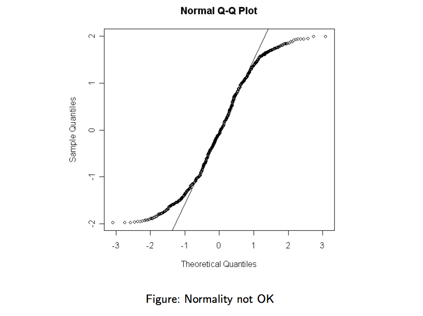
Such a plot is named a Q-Q Plot. We should see a diagonal line with -degrees angle. If the line significantly deviates from the -degrees line, there is evidence against the normality assumption. This easily reveals outliers, skewness and heaky tails.
Note: if we plot the empirical quantiles of the unstandardised residuals against those of a , then the line should have slope and intercept zero.
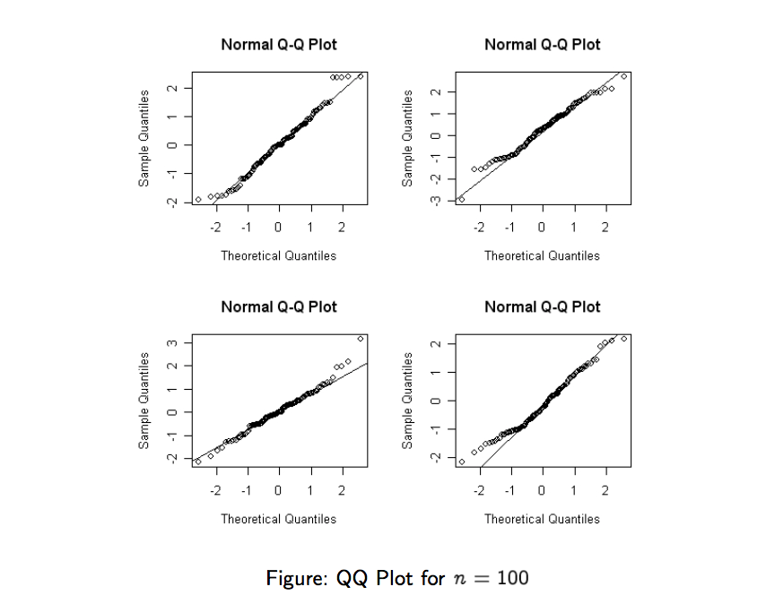
The lines won’t be perfect for small sample size, so don’t overinterpret the plot.
This is how a normal Q-Q plot looks like for a small sample :
And here is a Q-Q plot that invalidates the normality hypothesis:
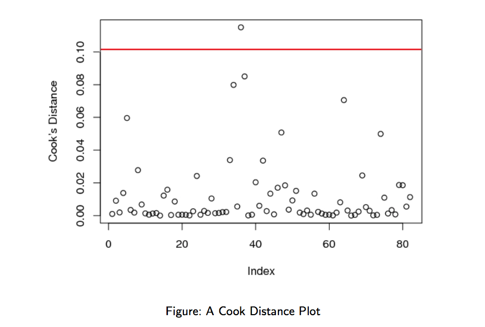
Checking for influential observations
How to know if a line in the design matrix has a strong influence on the fitted model? Remove the line and re-fit. Then compare with original model.
Let the output vector where row is removed and the design matrix where the -th row is removed. Note the estimated parameter vector in this new setup.
The Cook distance measures the scaled distance between the original estimate and the estimate of the truncated model :
As a rule of thumb, the rows () for which the cook distance is above the following threshold should be investiguated:
So let’s plot for each value of and compare with this threshold.