What is logistic regression?

A Logistic regression is a generalized linear model which is tailored to classification. In this article, we introduce this regression and explain its origin.

Setup

The dataset $\dataset$ of study consists of $\ndataset$ pairs of input vector $\inputvec_{\idataset}$ and output value $\outputval_{\idataset}$:

$$\dataset = \{\paren{\inputvec_{\idataset}, \outputval_{\idataset}} \mid \idataset \leq \ndataset\}$$

We suppose that there exists an approximate deterministic relationship $\truemodel$ between the inputs $\inputvec_{\idataset}$ and the outputs $\outputval_{\idataset}$:

$$\forall \idataset \leq \ndataset, \quad \outputval_{\idataset} \approx \truemodel\paren{\inputvec_{\idataset}}$$

The goal of a logistic regression is to learn this relationship using a subset $\trainset \subseteq \dataset$ of the dataset.

Generalized Linear models

We will approximate the relationship $\truemodel$ using the combination of a deterministic function $\logit$ and a linear model. This means that we want to find the best model $\bestmodel$ in the class $\linclass$ of linear models such that:

$$\logit\circ\bestmodel(\ninputvec{\idataset}) = \logit\paren{\bestmodel(\ninputvec{\idataset})} = \truemodel(\ninputvec{\idataset})$$

The inverse link function

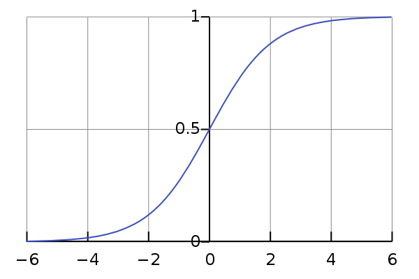
The deterministic function $\logit$ that we will use is the logistic function (we will explain why later):

$$\logit(x) = \frac{e^x}{1 + e^x}$$

Here is a graph of this function:

The logistic loss

To measure progress during learning, we use the logistic loss:

$$\begin{align*} \llogit(\linmodel{\linparamv}, \dataset) = - \sum_{\idataset = 1}^{\ndataset} \, \ln\paren{1 + e^{\linmodel{\linparamv}(\ninputvec{\idataset})}} - \ioutputval{\idataset}\,\linmodel{\linparamv}(\ninputvec{\idataset}) \end{align*}$$

Learning the best model then amounts to minimizing the training objective $\g$

Origin of the logistic loss

As discussed in this article, usual regression models are ill-adapted to classification.

Logistic regression, however, is tailored to classification problems: instead of directly attempting to predict the label $\outputval \in \{0, 1\}$, predict the probability $p(1 \mid \inputvec)$ that $\inputvec$ is in class $1$. That way, we turn a discrete classification problem into a continuous regression problem.

Since the values predicted by a regression model are in range $]-\infty;+\infty[$, there only remains to find a way to continuously shrink this range to $[0; 1]$. This can be done using the logistic function $\logit$, which is particularly interesting because most of the values it takes agglutinate around $0$ and $1$:

$$\logit(x) = \frac{e^x}{1 + e^x}$$

Here is a graph of this function:

Using the logistic function, we get the following expression for the probablity $p(1 \mid \inputvec)$ that $\inputvec$ is in class $1$:

$$p(1 \mid \inputvec) = \logit\paren{\linmodel{\linparamv}\cdot\inputvec}$$

And the probability $p(0 \mid \inputvec)$ that $\inputvec$ is in class $0$:

$$p(0 \mid \inputvec) = 1 - \logit\paren{\linmodel{\linparamv}\cdot\inputvec}$$

To predict the labels, we compare those probabilities to a threshold ($0.5$):

$$\hat{\ioutputval{\idataset}} = 1 \iff p(1 \mid \ninputvec{\idataset}) > 0.5$$

Learning the model’s parameters

So, our model predicts the probability $p(1 \mid \inputvec)$ that $\inputvec$ falls within class $1$. How do we learn its parameter vector $\linparamv$?

We will maximize the likelihood to obtain our data. Assuming that each training example $(\ninputvec{\idataset}, \ioutputval{\idataset})$ was drawn independently from the distribution $p$, the joint likelihood is:

$$p(\outputvec, \inputmatrix \mid \linparamv) = \prod_{\idataset = 1}^{\ndataset} p(\ioutputval{\idataset}, \ninputvec{\idataset} \mid \linparamv)$$

Which is maximal when the log-likelihood is:

$$\ln\circ\, p(\outputvec, \inputmatrix \mid \linparamv) = \sum_{\idataset = 1}^{\ndataset} \ln\circ\, p(\ioutputval{\idataset}, \ninputvec{\idataset} \mid \linparamv)$$

Where I use the notation $f \circ g(x) = f(g(x))$ for function composition.

For each $\idataset \leq \ndataset$, we have:

$$\begin{align*} p(\ioutputval{\idataset}, \ninputvec{\idataset} \mid \linparamv) &= p(\ioutputval{\idataset} \mid \ninputvec{\idataset}, \linparamv)\,p(\ninputvec{\idataset} \mid \linparamv) \end{align*}$$

Since:

$$\begin{align*} & \ioutputval{\idataset} = 1 \implies p(\ioutputval{\idataset} \mid \ninputvec{\idataset}, \linparamv) = \logit\paren{\linmodel{\linparamv}\cdot\ninputvec{\idataset}} \\ & \ioutputval{\idataset} = 0 \implies p(\ioutputval{\idataset} \mid \ninputvec{\idataset}, \linparamv) = 1 - \logit\paren{\linmodel{\linparamv}\cdot\ninputvec{\idataset}} \end{align*}$$

We find that:

$$\frac{p(\ioutputval{\idataset} \mid \ninputvec{\idataset}, \linparamv)}{p(\ninputvec{\idataset} \mid \linparamv)} = \ioutputval{\idataset}\,\logit\paren{\linmodel{\linparamv}\cdot\ninputvec{\idataset}} + \paren{1 - \ioutputval{\idataset}}\,\paren{1 - \logit\paren{\linmodel{\linparamv}\cdot\ninputvec{\idataset}}}$$

Since $p(\ninputvec{\idataset} \mid \linparamv)$ is a constant (the inputs does not depend on $\linparamv$), we find that the value to maximize is:

$$\sum_{\idataset = 1}^{\ndataset} \ioutputval{\idataset}\,\ln\circ\, \logit\paren{\linmodel{\linparamv}\cdot\ninputvec{\idataset}} + \paren{1 - \ioutputval{\idataset}}\,\paren{1 - \ln\circ\, \logit\paren{\linmodel{\linparamv}\cdot\ninputvec{\idataset}}}$$

Replacing $\logit$ by its definition and simplifying, we find the expression to maximize:

$$\sum_{\idataset = 1}^{\ndataset} \, \ln\paren{1 + e^{\linmodel{\linparamv}(\ninputvec{\idataset})}} - \ioutputval{\idataset}\,\linmodel{\linparamv}(\ninputvec{\idataset})$$

Which is precisely $- \llogit(\linmodel{\linparamv}, \dataset)$. Hence its use as loss function.

But…

The choice of $\logit$ might seem arbitrary. Is it a good idea to predict the probability $p(1 \mid \inputvec)$? What if we used another function to shrink $]-\infty;+\infty[$?

The theoretical soundness of the logistic regression is explained in the following section.

Logistic regression is a generalized linear model

Logistic regression is a generalized linear model with inverse link function:

$$\logit(x) = \frac{e^x}{1 + e^x}$$

The output $\linmodel{\linparamv}(\inputvec)$ of the linear regression is an estimate of the natural parameter $\eta$ of a Bernoulli($p$) distribution:

$$\eta = \logit^{-1}(p) = \ln\paren{\frac{p}{1 - p}}$$

Underlying probabilistic model

The underlying probabilistic model when using a logistic regression is thus:

Let $\rve{X}$ a random vector whose first component is always $1$ (this is our bias-term). Let $\linparamv_\text{true}$ be a vector and let $\rva{Y} \distributed Bern(p(\rve{X}))$ be a Bernoulli random variable with probability of success $p(\rve{X}) = \logit(\linparamv_\text{true} \cdot \rve{X})$.

Our dataset $S$ is made of $\ndataset$ i.i.d. samples from the random vector $(\rve{X}, \rva{Y})$:

$$S = \{(\ninputvec{\idataset}, \ioutputval{\idataset}) \iid (\rve{X}, \rva{Y}) \mid \idataset \leq \ndataset \}$$

Hence, for each $\idataset \leq \ndataset$, we know that $\ioutputval{\idataset}$ is an observation drawn from a $Bern(\logit(\linparamv_\text{true} \cdot \ninputvec{\idataset}))$ distribution.

In this setup, the logistic regression predicts the value of the natural parameter $\eta = \logit^{-1}(p(\ninputvec{\idataset}))$ so as to maximize the likelihood of the observed data.