A non-technical introduction to statistics

$\def\sa{a} \def\sb{b} \def\sc{c} \def\sd{d} \def\se{e} \def\sf{f} \def\sg{g} \def\sh{h} \def\si{i} \def\sj{j} \def\sk{k} \def\sl{l} \def\sm{m} \def\sn{n} \def\so{o} \def\sp{p} \def\sq{q} \def\sr{r} \def\ss{s} \def\st{t} \def\su{u} \def\sv{v} \def\sw{w} \def\sx{x} \def\sy{y} \def\sz{z} \def\va{\vec{a}} \def\vb{\vec{b}} \def\vc{\vec{c}} \def\vd{\vec{d}} \def\ve{\vec{e}} \def\vf{\vec{f}} \def\vg{\vec{g}} \def\vh{\vec{h}} \def\vi{\vec{i}} \def\vj{\vec{j}} \def\vk{\vec{k}} \def\vl{\vec{l}} \def\vm{\vec{m}} \def\vn{\vec{n}} \def\vo{\vec{o}} \def\vp{\vec{p}} \def\vq{\vec{q}} \def\vr{\vec{r}} \def\vs{\vec{s}} \def\vt{\vec{t}} \def\vu{\vec{u}} \def\vv{\vec{v}} \def\vw{\vec{w}} \def\vx{\vec{x}} \def\vy{\vec{y}} \def\vz{\vec{z}} \def\ga{\mathfrak{A}} \def\gb{\mathfrak{B}} \def\gc{\mathfrak{C}} \def\gd{\mathfrak{D}} \def\ge{\mathfrak{E}} \def\gf{\mathfrak{F}} \def\gg{\mathfrak{G}} \def\gh{\mathfrak{H}} \def\gi{\mathfrak{I}} \def\gj{\mathfrak{J}} \def\gk{\mathfrak{K}} \def\gl{\mathfrak{L}} \def\gm{\mathfrak{M}} \def\gn{\mathfrak{N}} \def\go{\mathfrak{O}} \def\gp{\mathfrak{P}} \def\gq{\mathfrak{Q}} \def\gr{\mathfrak{R}} \def\gs{\mathfrak{S}} \def\gt{\mathfrak{T}} \def\gu{\mathfrak{U}} \def\gv{\mathfrak{V}} \def\gw{\mathfrak{W}} \def\gx{\mathfrak{X}} \def\gy{\mathfrak{Y}} \def\gz{\mathfrak{Z}} \def\ra{A} \def\rb{B} \def\rc{C} \def\rd{D} \def\re{E} \def\rf{F} \def\rg{G} \def\rh{H} \def\ri{I} \def\rj{J} \def\rk{K} \def\rl{L} \def\rm{M} \def\rn{N} \def\ro{O} \def\rp{P} \def\rq{Q} \def\rr{R} \def\rs{S} \def\rt{T} \def\ru{U} \def\rv{V} \def\rw{W} \def\rx{X} \def\ry{Y} \def\rz{Z} \def\rva{\vec{A}} \def\rvb{\vec{B}} \def\rvc{\vec{C}} \def\rvd{\vec{D}} \def\rve{\vec{E}} \def\rvf{\vec{F}} \def\rvg{\vec{G}} \def\rvh{\vec{H}} \def\rvi{\vec{I}} \def\rvj{\vec{J}} \def\rvk{\vec{K}} \def\rvl{\vec{L}} \def\rvm{\vec{M}} \def\rvn{\vec{N}} \def\rvo{\vec{O}} \def\rvp{\vec{P}} \def\rvq{\vec{Q}} \def\rvr{\vec{R}} \def\rvs{\vec{S}} \def\rvt{\vec{T}} \def\rvu{\vec{U}} \def\rvv{\vec{V}} \def\rvw{\vec{W}} \def\rvx{\vec{X}} \def\rvy{\vec{Y}} \def\rvz{\vec{Z}} \def\seta{A} \def\setb{B} \def\setc{C} \def\setd{D} \def\sete{E} \def\setf{F} \def\setg{G} \def\seth{H} \def\seti{I} \def\setj{J} \def\setk{K} \def\setl{L} \def\setm{M} \def\setn{N} \def\seto{O} \def\setp{P} \def\setq{Q} \def\setr{R} \def\sets{S} \def\sett{T} \def\setu{U} \def\setv{V} \def\setw{W} \def\setx{X} \def\sety{Y} \def\setz{Z} \def\fa{a} \def\fb{b} \def\fc{c} \def\fd{d} \def\fe{e} \def\ff{f} \def\fg{g} \def\fh{h} \def\fi{i} \def\fj{j} \def\fk{k} \def\fl{l} \def\fm{m} \def\fn{n} \def\fo{o} \def\fp{p} \def\fq{q} \def\fr{r} \def\fs{s} \def\ft{t} \def\fu{u} \def\fv{v} \def\fw{w} \def\fx{x} \def\fy{y} \def\fz{z} \def\fA{A} \def\fB{B} \def\fC{C} \def\fD{D} \def\fE{E} \def\fF{F} \def\fG{G} \def\fH{H} \def\fI{I} \def\fJ{J} \def\fK{K} \def\fL{L} \def\fM{M} \def\fN{N} \def\fO{O} \def\fP{P} \def\fQ{Q} \def\fR{R} \def\fS{S} \def\fT{T} \def\fU{U} \def\fV{V} \def\fW{W} \def\fX{X} \def\fY{Y} \def\fZ{Z} \def\ma{A} \def\mb{B} \def\mc{C} \def\md{D} \def\me{E} \def\mf{F} \def\mg{G} \def\mh{H} \def\mi{I} \def\mj{J} \def\mk{K} \def\ml{L} \def\mm{M} \def\mn{N} \def\mo{O} \def\mp{P} \def\mq{Q} \def\mr{R} \def\ms{S} \def\mt{T} \def\matu{U} \def\mv{V} \def\mw{W} \def\mx{X} \def\my{Y} \def\mz{Z} \def\loss{\mathcal{L}} \newcommand{\dkl}[2]{D_{\text{KL}}\mathopen{}\paren{#1\,||\,#2}} \newcommand{\dataset}{S} \newcommand{\ndataset}{N} \newcommand{\idataset}{n} \newcommand{\inputRV}{\mathcal{X}} \newcommand{\inputvec}{\vec{x}} \newcommand{\ninputvec}[1]{\vec{x}_{#1}} \newcommand{\iinputvec}[1]{x_{#1}} \newcommand{\niinputvec}[2]{x_{#1, #2}} \newcommand{\icpnt}{i} \newcommand{\inputmatrix}{X} \newcommand{\inputdim}{D} \newcommand{\outputval}{y} \newcommand{\ioutputval}[1]{y_{#1}} \newcommand{\outputvec}{\vec{y}} \newcommand{\trainset}{S_{\text{train}}} \newcommand{\testset}{S_{\text{test}}} \newcommand{\truemodel}{f_{\text{true}}} \newcommand{\trainedmodel}{f_{\trainset}} \newcommand{\linmodel}[1]{f_{#1}} \newcommand{\bestmodel}{f^{*}} \newcommand{\model}{f} \newcommand{\hyperparam}{\lambda} \newcommand{\linparamv}{\vec{w}} \newcommand{\ilinparam}[1]{w_{#1}} \newcommand{\indivloss}{l} \newcommand{\modelclass}{\mathcal{F}} \newcommand{\linclass}{\modelclass_{\text{lin}}} \newcommand{\g}{\mathcal{G}} \newcommand{\gmse}{\g_{\text{MSE}}} \newcommand{\glasso}{\g_{\text{lasso}}} \newcommand{\gridge}{\g_{\text{ridge}}} \newcommand{\glogit}{\g_{\logit}} \newcommand{\l}{\mathcal{L}} \newcommand{\lmse}{\l_{\text{MSE}}} \newcommand{\lmae}{\l_{\text{MAE}}} \newcommand{\llasso}{\l_{\text{lasso}}} \newcommand{\lridge}{\l_{\text{ridge}}} \newcommand{\llogit}{\l_{\logit}} \newcommand{\logit}{\sigma} \newcommand{\reg}{\mathcal{R}} \DeclareMathOperator*{\argmin}{argmin} \DeclareMathOperator*{\argmax}{argmax} \DeclareMathOperator*{\mean}{mean} \DeclareMathOperator*{\avg}{avg} \DeclareMathOperator*{\span}{span} \DeclareMathOperator*{\var}{var} \DeclareMathOperator*{\bias}{bias} \newcommand{\expectation}{\mathbb{E}} \newcommand{\brak}[1]{\left[#1\right]} \newcommand{\paren}[1]{\left(#1\right)} \newcommand{\realset}{\mathbb{R}} \newcommand{\realvset}[1]{\realset^{#1}} \newcommand{\prob}{\mathbb{P}} \newcommand{\gaussian}{\mathcal{N}} \newcommand{\iid}{\stackrel{\text{i.i.d.}}{\sim}} \newcommand{\abs}[1]{\left\lvert#1\right\rvert} \newcommand{\norm}[1]{\left\lVert#1\right\rVert} \newcommand{\normtwo}[1]{\norm{#1}_{2}} \newcommand{\normone}[1]{\norm{#1}_{1}} \newcommand{\card}[1]{\left\lvert#1\right\rvert} \newcommand{\grad}{\nabla} \newcommand{\dconv}{\stackrel{d}{\to}} \newcommand{\pconv}{\stackrel{p}{\to}} \newcommand{\rva}[1]{#1} \newcommand{\rve}[1]{\vec{#1}} \newcommand{\obs}[1]{#1} \newcommand{\vobs}[1]{\vec{#1}} \newcommand{\distrib}[1]{#1} \newcommand{\distribof}[2]{#1_{#2}} \newcommand{\density}[1]{#1} \newcommand{\densityof}[2]{#1_{#2}} \newcommand{\distributed}{\sim} \newcommand{\const}[1]{#1} \newcommand{\fun}[1]{#1}$

This article explains in simple terms the purpose of statistical theory and gives an overview of how it is used.

Statistics is a branch of mathematics composed of two aspects: descriptive statistics and statistical inference.

Descriptive statistic can be assimilated to a language used to summarize data. For instance, mean and average are words from the descriptive statistics lexicon.

Statistical inference is the clever part of statistics: when we are interested in some feature of a large population we usually can’t examine every member of the population, so we take a random sample and use this incomplete information to make reasonable guesses about the population. The whole purpose of the theory is to quantify what reasonable guesses are and under what circumstances they hold.

Statistical inference: sample data ⟹ probability model

We may at once admit that any inference from the particular to the general must be attended with some degree of uncertainty, but this is not the same as to admit that such inference cannot be absolutely rigorous, for the nature and degree of the uncertainty may itself be capable of rigorous expression. – Ronald A. Fisher

Non-technical overview

I will now illustrate how we can use statistical inference to gain knowledge about a population. I removed most technical developments from the exposition. Also, I deliberately used some statistical terms such as sample and parameter so that this example serves as a first introduction to the statistical lexicon. You should pay attention to the mathematical letters such as $\bar{X}$ . There are few of them and they are often repeated in the text to ease their memorization. They come in handy for more involved explainations.

To illustrate the process, suppose that you have a general population P. For instance, this population can be the heights of all US citizens, which is set of number. Suppose we want to gain knowledge about a population parameter. For instance, the mean of those heights.

Since we can’t measure everyone in America, we will restrict ourselves to a random sample, which means we randomly choose a given number (note this number $n$ ) of people and we measure them. This gives us $n$ numbers $X_1, ..., X_n$ that we call the sample. As a shorthand, I will use the notation: $(X)_{1}^{n} = X_1, ..., X_n$

Statistics uses several approaches and tools to learn about the population parameter from our sample $(X)_{1}^{n}$ . There are three approaches:

point estimates;
confidence intervals;
hypothesis testing.

Actually, point 1 and 2 are very similar so there really only two approaches.

A distinction without a difference has been introduced by certain writers who distinguish “Point estimation”, meaning some process of arriving at an estimate without regard to its precision, from “Interval estimation” in which the precision of the estimate is to some extent taken into account. – R. A. Fisher (1956)

1. Point estimates

We can estimate the parameter by its statistical counterpart in the sample. Thus, for instance, we would estimate the population mean $\bar{P}$ by the sample mean $\bar{X}$ . We don’t know what the real population mean is because we can’t measure everyone, but we can compute the mean of our sample $(X)_{1}^{n}$ .

The question is: how are the population mean $\bar{P}$ and the sample mean $\bar{X}$ related? A priori, nothing tells us that they should be equal. Maybe our sample mean will be very different from the total population mean. If you have trouble visualising this, imagine that our random sample yields the heights of 100 US-citizens aged between 2 and 5 years old… Your sample mean is likely to be well under the population mean.

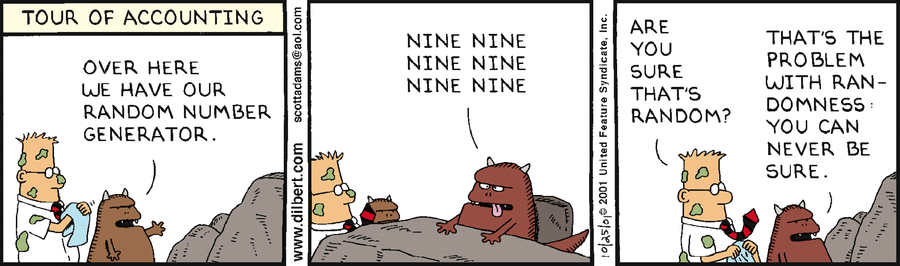Randomness Comics by dilbert

Notice that if we took a number of different samples, each of size $n$ , from the population, we would get a different sample mean $\bar{X}$ each times. So, if we collect different samples and they usually give us different results, how can we make any inference about the population?

The key insight is that even though the values of the statistic are likely to differ from sample to sample, they will follow a pattern. This pattern is called the sampling distribution. In formal terms, the sampling distribution of a statistic is the probability distribution for the set of possible values that can be assumed by the statistic. If you don’t know what a distribution is, read my dedicated article: Introduction to data distributions (to be redacted).

So, in order to know if our estimator is a good, we focus our study on the distribution of the estimator accross different sample. If we took many samples, would their means average out to the true population mean $\bar{P}$ ? And if so, how close to the population mean $\bar{P}$ will our sample mean $\bar{X}$ typically be?

In statistical terms, both questions are about the sampling distribution of our estimator $\bar{X}$ :

Where is the sampling distribution of $\bar{X}$ centered?
How does the variability of $\bar{X}$ across samples compare to the variability in the population?

In the well studied case of means, statistical theory answers yes to the first question. The sample means average out to the population mean $\bar{P}$ , or in other words: our sampling distribution is centered at the population mean $\bar{P}$ . We say that our estimator is unbiased.

As a side note, remark that we could very well use an element from the sample as our estimator, instead of the whole sample’s mean. In that case, we can show that this new estimator is unbiased too. But it’s less interesting because the confidence interval that we can attach to it is less precise than that of the mean estimator, because it fails to take additional information into account as the size of the sample grows. See below to learn about confidence intervals.

Regarding the second question, theory also tells us that the bigger our sample size, the closer to the population mean $\bar{P}$ our sample mean $\bar{X}$ will be. This makes sense, since as the sample size grows we incorporate more and more information from the population.

So far, we know that we can estimate the population mean using our sample mean, and we know that the bigger the sample, the more precise our estimation will be. But how precise exactly?

2. Confidence intervals

We can use the sampling distribution once again to establish confidence intervals. It is a statement such as:

The average height of males in the US is 175cm +/- 6.2cm

What does it mean? And how do we compute the interval?

What is a confidence interval?

Since confidence intervals are used everywhere (on the news, on the internet, etc.), we will take the time to clearly define what they mean.

If we have 95% confidence interval for a population parameter, this means that 95% of all possible random samples will yield data for which the interval contains the population parameter. The remaining 5% of the random samples will yield data for which it doesn’t. So, once the random sample is chosen, there are no probabilities: either the sample yields an interval that contains the parameter, or it doesn’t.

Confidence intervals qualify the sampling process. You have 95% chance to choose a sample yielding a confidence interval that actually contains the parameter. And you have 5% chance to choose a sample that doesn’t.

For instance, if the 95% confidence interval is +/-6.2cm, then we have 95% chance to choose a sample such that the mean height $\bar{P}$ of the total population satisfies:

\[\bar{X} - 6.2cm \leq \bar{P} \leq \bar{X} + 6.2cm\]

Where $\bar{X}$ is our sample mean as previously defined.

How do we compute confidence intervals?

to be continued