The geometry of (normal) parameter estimation

This article shows geometrically where the best estimates for the mean and variance of a normally distributed random vector can be found. We start with a simple question and derive both the geometrical meaning and parameter estimation method from scratch.

Goal

If you’re impatient to know where we’re headed, here are the geometrical insights we will develop in this article:

1) Given $2$ observations $y_1$ and $y_2$ independently generated at random by the distribution $\mathcal{N}(\mu, \sigma)$, our best estimators for $\mu$ and $\sigma$ are $\hat{\mu}$ and $\hat{\sigma}$ such that:

$$\begin{pmatrix}y_1 \\ y_2\end{pmatrix} = \hat{\mu}\,\begin{pmatrix}1\\1\end{pmatrix} + \frac{\hat{\sigma}}{\sqrt{2}}\,\begin{pmatrix}-1 \\ 1 \end{pmatrix}$$

2) More generally, given $n$ observations $\vec{y}_n = (y_1, ..., y_n)$ independently generated at random by the same distribution $\mathcal{N}(\mu, \sigma^2)$, our best estimators are:

$$\vec{y}_n = \hat{\mu}\,(\sqrt{n}\,\mathbb{U}_n) + \hat{\sigma}\,(\sqrt{n-1}\,\mathbb{U}_n^{\perp})$$

where $\sqrt{n}$ and $\sqrt{n-1}$ are correction factors because as dimension increases, distances increases. The meaning of $\mathbb{U}_n$ and $\mathbb{U}_n^{\perp}$ are illustrated on the picture below:

Introduction

We can think of a probability distribution as an engine able to generate values at random. A random vector is a vector whose components have been generated by such engine.

Conceptually, it is useful to see the density function for a random vector as a cloud in $R^n$ that indicates the plausible end points for the random vector: the vector is more likely to end in a region where the cloud is dense than one where it is not dense.

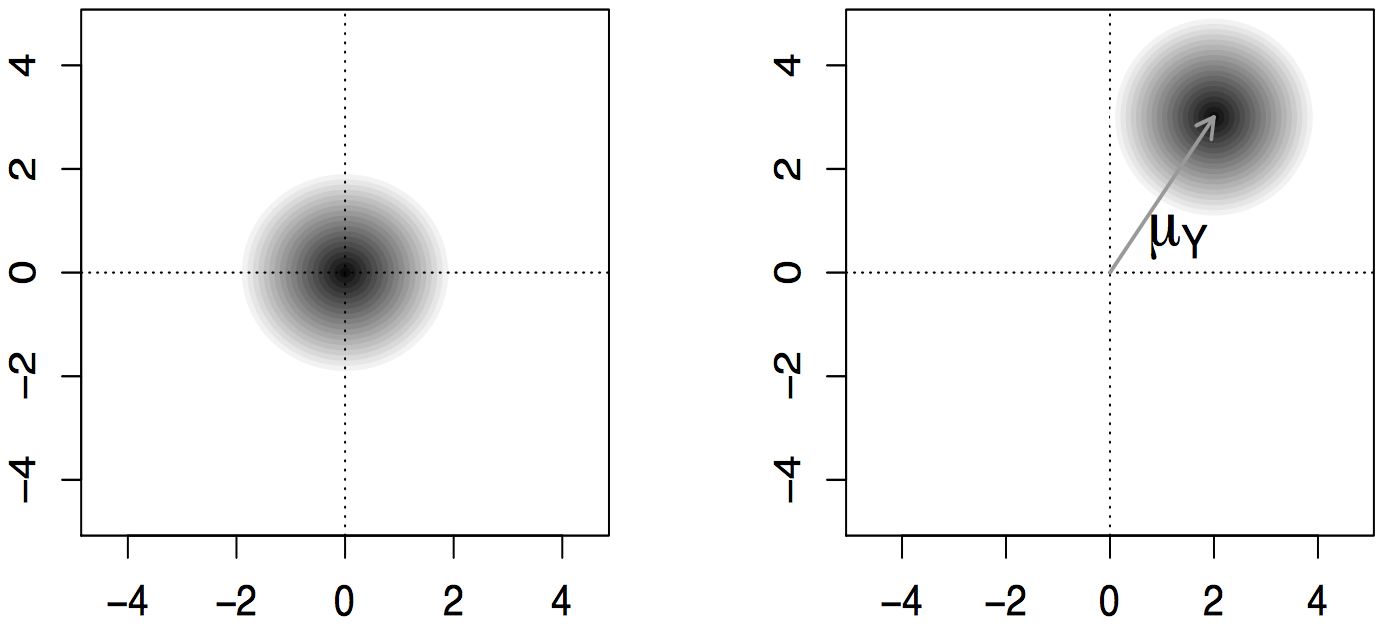Figure. Density cloud for a vector with $\mathcal{N}(\vec{0}, \sigma^2)$ distribution on the left and $\mathcal{N}(\vec{\mu_Y}, \sigma^2)$ distribution on the right.

For instance, the following image shows the “density cloud” of a normally distributed random vector. The components of the vector are generated by a normal distribution, and the visualization shows how this translate to 2D geometry.

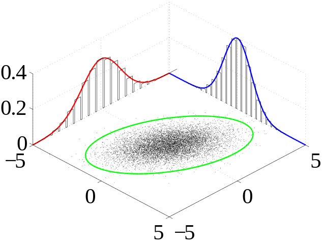
Here, the shape of the “density cloud” for the random vector is determined by the parameters of each component: the shape of a normal distribution is controlled by the mean $\mu$ (= location of the center) and it’s variance $\sigma^2$ (= size of the cloud). When the variance for every component is the same, the cloud is a circle.

The shape of the normal distribution (or gaussian distribution) is particularly interesting because it models measurement errors. We can think of it as a cloud that generates a target value $\mu$ with some measurement noise. The variance parameter $\sigma^2$ controls the amount of noise that is added. Among all its desirable features, the distribution is symetric: accross a very large number of measurement, we expect the errors to cancel each others, so that the mean of the sample approximates the real value $\mu$. We will see later that it has a nice geometrical feature too.

To learn more about the normal distribution, check out this article: A probability distribution to model measurement errors.

Statistics is all about finding the location of the cloud when we have a few observations but we don’t know the parameters $\mu$ and $\sigma$. As we will see, the normal distribution has a nice property that allows us to visualize geometrically the process of estimating those parameters.

Finding the cloud

Suppose for instance that we have two observations $y_1$ and $y_2$ independently generated at random by the same normal distribution $\mathcal{N}(\mu, \sigma^2)$.

We would like to estimate the most likely values for the parameters of the cloud: its center $\mu$ and it’s standard deviation $\sigma$. Basically, this means that we will try to find the “best guess” for those values based on the location of our observations.

Our best guess for the center is to place it where it has the highest probability to generate our observations. In statistical terms, we are looking for the maximum likelihood value of $\mu$.

To find this maximum likelihood location, we need to study the formula for the could’s density more closely.

$$f(Y = y \mid \mu, \sigma) = \frac{1}{\sqrt{2\pi\sigma^2}}\mathrm{exp}(-\frac{\left|y-\mu\right|^2}{2\sigma^2})$$

Since both observations are generated independently, the joint density (= the density for both) is the product $f(Y_1 = y_1 \mid \mu, \sigma)\,f(Y_2 = y_2 \mid \mu, \sigma)$ which is maximal when $\mu$ minimizes this sum:

$$\hat{\mu} = \mathrm{argmin}_{\mu} (y_1 - \mu)^2 + (y_2 - \mu)^2$$

You might recognize the Ordinary Least Square equation. This sum has a nice geometrical interpretation because it is exactly the expanded formula for the norm (= length) of the vector $\vec{y} - (\mu, \mu)$:

$$\hat{\mu} = \mathrm{argmin}_{\mu} \left\lVert\begin{pmatrix}y_1 \\ y_2\end{pmatrix} - \mu\,\begin{pmatrix}1\\1\end{pmatrix}\right\rVert^2$$

Geometry

So we are looking for the point on the line of direction $(1, 1)$ that is the closest to $\vec{y} = (y_1, y_2)$.

This point is the orthogonal projection of $\vec{y}$ onto the unit vector $\vec{u}$ directed along the line. We can use the dot product $\cdot$ to find the projection coefficient, and multiply by the unit vector to get the projection:

$$\hat{\mu}\begin{pmatrix}1\\1\end{pmatrix} = (\vec{y}\cdot\vec{u})\,\vec{u} \quad \text{(equation 1)}$$

Yeay! We found our best estimate for the center of the cloud!

To ease the transition with higher dimensions, let’s shorten our notation for the vector $(1,1)$ as $\mathbb{I}_2$ where the number $2$ stands for the number of components in the vector. So that for instance, $\mathbb{I}_4 = (1,1,1,1)$. Geometrically, we can see this vector as the diagonal of the $n$-dimensional (hyper)cube of side $1$. The norm of this vector is simply the length of that diagonal: $\lVert\mathbb{I}_2\rVert = \sqrt{2}$ or more generally, $\lVert\mathbb{I}_n\rVert = \sqrt{n}$. This will prove useful later.

Likewise, let’s adopt a more flexible notation for our unit vector $\vec{u}$ and use $\mathbb{U}_2$ for the unit vector directed along $\mathbb{I}_2$. In math notations, this means that: $\mathbb{I}_n = \sqrt{n}\,\mathbb{U}_n$ for all values of $n$. Since $\mathbb{U}_n$ is a unit vector, we can use it to express the orthogonal projection of $\vec{y}$. With these notations equation 1 becomes:

$$\hat{\mu}\,\mathbb{I}_2 = (\vec{y}\cdot\mathbb{U}_2)\,\mathbb{U}_2$$

This is a vector equation. Let’s find the exact value of our estimate:

$$\begin{eqnarray*} & \hat{\mu}\,\mathbb{I}_2 & = (\vec{y}\cdot\mathbb{U}_2)\,\mathbb{U}_2 \\ \iff & \hat{\mu}\,\sqrt{2}\,\mathbb{U}_2 & = (\vec{y}\cdot\mathbb{U}_2)\,\mathbb{U}_2 \\ \iff & \hat{\mu}\,\sqrt{2} &= (\vec{y}\cdot\mathbb{U}_2)\\ \iff & \hat{\mu} & = (\vec{y}\cdot\mathbb{U}_2)\,\frac{1}{\sqrt{2}}\\ \end{eqnarray*}$$

We can rewrite this slightly to get the ordinary least square solution $\hat{\mu} = \bar{y}$:

$$\begin{eqnarray*} && \hat{\mu} & = (\vec{y}\cdot\mathbb{U}_2)\,\frac{1}{\sqrt{2}}\\ &\iff & \hat{\mu} & = (\vec{y}\cdot\frac{\mathbb{I}_2}{\sqrt{2}})\,\frac{1}{\sqrt{2}}\\ &\iff & \hat{\mu} & = (\vec{y}\cdot\mathbb{I}_2)\,\frac{1}{2}\\ &\iff & \hat{\mu} & = \frac{y_1 + y_2}{2} \end{eqnarray*}$$

This result generalizes easily for a higher number of observations. Suppose for instance that $n$ stands for a positive integer and that we have $n$ observations $y_1$, …, $y_n$ independently generated at random by a normal distribution $\mathcal{N}(\mu, \sigma^2)$. If we write $\vec{y}_n = (y_1, ..., y_n)$ the random vector associated with our observations, we can find our best guess for the center of the cloud by projecting $\vec{y}_n$ onto $\mathbb{U}_n$. This yields the following best guess for $\mu$:

$$\hat{\mu} = (\vec{y}_n\cdot\mathbb{U}_n)\,\frac{1}{\sqrt{n}}= \frac{y_1 + ... + y_n}{n}$$

From now on, I will use the general notation with $n$ to make clear that our results hold in higher dimensions. While reading, feel free to consider that $n = 2$ or $n = 3$ to visualize the geometry.

Before we estimate the second parameter $\sigma$, let’s write $\vec{y}_n$ as the sum of the cloud’s center and a deviation vector $\vec{\epsilon}_n$ from the center. It that can be considered as if its components where independently generated at random by a $\mathcal{N}(0, \sigma^2)$ distribution.

$$\vec{y}_n = \hat{\mu}\,(\sqrt{n}\,\mathbb{U}_n) + \vec{\epsilon}_n$$

Now, I will do a few tricks to show that $\vec{\epsilon}_n$ can be used to estimate the standard deviation parameter $\sigma$. Once done, we will revert back to the geometrical interpretation.

Take $n - 1$ unit vectors to form a basis ($\mathbb{U}_n$, $u_1$, …, $u_{n-1}$) of space. This means we take a set of $n$ axis for space where $\mathbb{U}_n$ is the first of them. Note $Y_n$ the general random vector which has been realized as $\vec{y}_n$. Along each of those new unit vectors, the projection $Y_N\cdot u_i$ has $0$ mean and is distributed according to a normal distribution $\mathcal{N}(0, \sigma^2)$. We will show that the projection of $\vec{y}_n$ onto each of those directions yield an unbiased estimator for the variance $\sigma^2$. Indeed:

$$\begin{align*} \sigma^2 &= \mathrm{var}(Y_n\cdot u_i )\\ &= \mathbb{E}[\,(Y_n\cdot u_i )^2\,] - \mathbb{E}[\,Y_n\cdot u_i \,]^2 \\ &= \mathbb{E}[\,(Y_n\cdot u_i )^2\,] - 0 \\ &= \mathbb{E}[\,(Y_n\cdot u_i )^2\,] \end{align*}$$

We can pool these to get the best estimate for $\sigma^2$:

$$\hat{\sigma}^2 = \frac{\sum_{i = 1}^{n-1} (\vec{y}_n\cdot u_i)^2}{n-1} = \frac{\lVert\vec{\epsilon}_n\rVert^2}{n-1}$$

If take a unit vector $\mathbb{U}_n^{\perp}$ directed along $\vec{\epsilon}_n$, we know that it is orthogonal to $\mathbb{U}_n$ (hence the notation). And we have $\lVert\vec{\epsilon}_n\rVert\ = (\vec{y}_n\cdot\mathbb{U}_n^{\perp})$. Hence, our best estimate for the standard deviation $\sigma$ is:

$$\begin{align*} \hat{\sigma} = \frac{\lVert\vec{\epsilon}_n\rVert}{\sqrt{n-1}} = \frac{\vec{y}_n \cdot \mathbb{U}_n^{\perp}}{\sqrt{n-1}} \\ \end{align*}$$

In words, the standard deviation is the length of the deviation vector $\epsilon_n$ corrected for the dimension $n$. As I will explain later, this is because lengths are dilated in higher dimensions.

We can replace $\vec{\epsilon}$ by the above expression in the formula for the observation vector $\vec{y}_n$:

$$\vec{y}_n = \hat{\mu}\,(\sqrt{n}\,\mathbb{U}_n) + \hat{\sigma}\,(\sqrt{n-1}\,\mathbb{U}_n^{\perp})$$

The values $\sqrt{n}$ and $\sqrt{n-1}$ are scale factors due to the dimension of space. Indeed, the length of the diagonal of a square with size $s$ is: $\sqrt{2}\,s$, for a cube it is $\sqrt{3}\,s$ and more generally for a $n$-dimensional hypercube it is $\sqrt{n}\,s$. This explains the $\sqrt{n}$ factor associated with $\mathbb{U}_n$ which is precisely the direction of that diagonal.

Another way to say this is simply that $\sqrt{n}$ is the norm of $\mathbb{I}_n$ in the $n$-dimensional space.

Likewise, $\sqrt{n-1}$ is the norm of $\mathbb{I}_n^{\perp}$ in the $(n-1)$-dimensional subspace orthogonal to $\mathrm{span}(\mathbb{I}_n)$. We loose one dimension because $\epsilon$ can’t have any component colinear to $\mathbb{I}_n$ by definition.

In the special case when the components of $\epsilon$ are perfect estimators (i.e. when $\epsilon = (\sigma, ..., \sigma)$), the picture reduce to a true $(n-1)$-dimensional hypercube and $\sqrt{n-1}\,\sigma$ is its diagonal.

When $n=1$, we have only one observation ($y_1$) and the formula says that our best estimate for the parameter $\mu$ is:

$$y_1 = \hat{\mu} \sqrt{1} + \hat{\sigma} \sqrt{0} = \hat{\mu}$$

Which means that with only one value, our best guess is to center the distribution on that value. We don’t have enough observations to estimate $\sigma,$ so it is automatically ruled out of the formula.