Key ideas in probability and statistics illustrated on a simple problem

This article aims to illustrate what are probability theory and statistical inference in simple terms using a simple to understand problem: drawing colored balls from an urn.

Suppose that you have an urn containing red and green balls that you can’t distinguish otherwise than by their color. You can’t see inside the urn and you draw a ball without looking. Will you get a red or a green ball?

We don’t know if you will get a red ball or a green ball. But if there are a thousand green balls and only one red ball, then it’s very likely that you will get a green ball. But how likely exactly?

Probability theory aims to give a quantitative answer to that question. Given a problem as stated above, probability theory gives you the probability for a given outcome. The probability that you can compute for the outcome may or may not be useful for predicting the actual outcome. It’s usefulness primarily depends on how much you know about the problem.

For instance, if you don’t know anything about the urn except that it contains undistinguishable green and red balls, then there is no reason to expect a green ball more than a red ball. On the other hand, if there are more green balls than red balls, there’s good intuitive reason than the probability for drawing a green ball is greater than that of drawing a red ball.

So that’s the goal of probability theory. Probability theory starts with knowledge and gives you a probability measure for potential outcomes. We shall see later in this article how exactly the probabilities are computed and how we can use them to gauge our expectations.

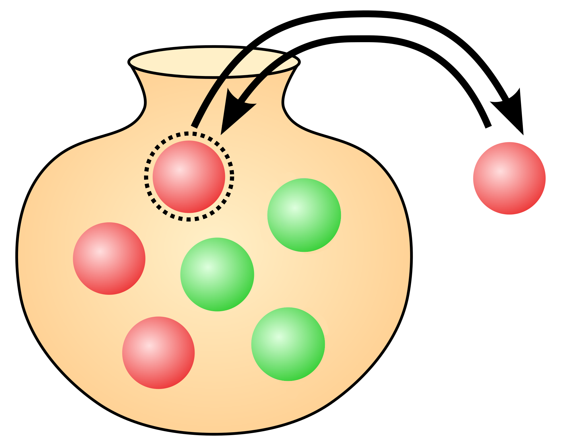
Statistical inference is concerned with the reverse problem: you have an urn containing red and green balls and you want to know the proportion of red balls. Of course, if the urn is small you can take every ball out and count the number of reds. But if the urn is very large, and if your time is limited, you won’t be able to count every balls. So what can you do?

The method in statistics is to draw a few balls from the urn. For instance, you take out 50 balls. This is called a sample of 50 balls. Then, you study the proportion of red balls in the sample and use it to draw estimates about the real proportion in the urn. You do so by estimating a probability measure that could have yielded the sample. So in a way, statistical inference is the reverse of probability theory: it starts with outcomes and ends with knowledge.

In the following exposion, we will survey the whole mathematical machinery required to solve both problems. For this purpose, we need first to define the rules of probability theory, and apply them to our urn problem. Then, we will take our second problem and go the other way around using statistical methods.

Probability theory: quantifying knowledge

My goal here is not to give a complete and rigorous construction of probability theory. Instead, I will give the most important rules and explain what they correspond to and how we can use them. We will then illustrate their use on our urn problem.

There are several constructions of probability theory, based on various mathematical objects (for instance, sets or propositions). These constructions differ in their philosophical view, but they all yield the same rules to compute probabilities, which in practice is what really matters.

Here are the rules. If you already know them, feel free to jump to the next section.

We will use capital letters to denote propositions. For instance: $B$ = “There is an urn. It contains red and green undistinguishable balls. We can’t see the color of a ball before taking it out from the urn”. Another example: $R$ = “My next draw from the urn yields a red ball”. The proposition can be true or false. For instance, I can draw a red ball from the urn, and $R$ was true. Or I could have drawn a green ball and $R$ was false.

Before I draw a ball, I don’t know whether $R$ is true or false. But I can measure my confidence that it will be true. We will measure our confidence in percent ($\%$) and use the following notation:

$$p(R\mid B) = 1.00 = 100\%$$

To say that we are $100\%$ confident that $R$ is true given our prior information $B$. To be clear, this means that we know $B$ is true and that we estimate our confidence in $R$ as $100\%$.

Or we can be only $50\%$ confident that $R$ is true, and in that case we note:

$$p(R\mid B) = .50 = 50\%$$

If I have more information about the problem, this can update my confidence estimate. For instance, if I know that the proposition $O$ = “There are only red balls left in the urn” is true, then I’m becoming $100\%$ confident that I will get a red ball. Which we note:

$$p(R\mid O, B) = 1.00$$

Notice how we take new information into account by inserting it after the vertical dash $\mid$.

Given a proposition, I can write a bar on top of it to say the opposite. For instance $\bar{R}$ = “My next draw from the urn does not yield a red ball”. I can estimate my confidence in $\bar{R}$ from my confidence in $R$:

$$p(\bar{R} \mid B) = 1.00 - p(R) = 100\% - p(R)$$

Which makes sense because if I’m $100\%$ confident that $R$ is true, then I’m $0\%$ confident that it is false. In other words, I’m $0\%$ confident that $\bar{R}$ is true.

Given a second proposition, for instance $R_2$ = “My second next draw from the urn yield a red ball”, I can estimate my confidence that both $R$ and $R_2$ will be true like this:

• first I estimating my confidence in one: $p(R \mid B)$
• then, I consider it true and estimate my confidence in the other: $p(R_2 \mid R, B)$.

So, if we note $R \& R_2$ the proposition stating that both $R$ and $R_2$ are true, I can estimate my confidence in it by:

$$p(R \& R_2 \mid B) = p(R \mid B)\cdot p(R_2 \mid R, B)$$

Or, I can do it the other way around:

$$p(R \& R_2 \mid B) = p(R_2 \mid B)\cdot p(R \mid R_2, B)$$

Where the dot is used to mean “multiplication”.

Having established these two rules, I can compute my estimate that one of $R$ or $R_2$ is true using the logic formula for “or”: $R \lor R_2 = \neg(\bar{R} \& \bar{R_2})$. If you don’t know what this formula means, don’t worry. The only thing you need is the resulting rule for computing the estimate of ($R$ or $R_2$) that we note $R \lor R_2$:

$$p(R \lor R_2 \mid B) = p(R \mid B) + p(R_2 \mid B) - p(R \& R_2 \mid B)$$

Let’s put this formula to test with some numerical values. Before that, let’s suppose that our estimate for $R_2$ does not depend on $R$. That is, our confidence in $R_2$ will be the same, whether we know $R$ is true or not. We can note this in the theory simply by assigning the same value for $p(R_2 \mid B)$ and $p(R_2 \mid R, B)$.

description	estimate	value
estimate in $R$	$p(R \mid B)$	$100\%$
estimate in $R_2$	$p(R_2 \mid B)$	$1\%$
same when we know $R$	$p(R_2 \mid R, B)$	$1\%$
use formula for “and”	$p(R \& R_2 \mid B)$	$100\% \cdot 1\% = 1\%$
use formula for “or”	$p(R \lor R_2 \mid B)$	$100\% + 1\% - 1\% = 100\%$

So, if I’m very confident in $R$ but not confident in $R_2$, probability theory says that I should be very confident that either $R$ or $R_2$ is true, since $p(R \lor R_2 \mid B) = 100\%$. It also says that I should not be confident that both $R$ and $R_2$ are true since $P(R \& R_2 \mid B) = 100\%$. Which make intuitive sense when you think about it.

Application to our urn problem

We will now use probability theory to estimate what we can expect when we draw colored balls from an urn. This looks like a toy problem but many fundamental aspects of probability theory and methodology can be illustrated with it.

Equiprobability from symmetry argument

As previously, let $B$ be the background information stating our problem: $B$ = “There is an urn. It contains red and green undistinguishable balls. We can’t see the color of a ball before taking it out from the urn”.

The question of interest is: “What is our confidence that we will draw a red ball?”

With our current state of knowledge, there is no reason to expect a red ball more than a green ball. A symmetry argument can help us see why: since the information about the color “red” and the color “green” are completely symmetric in $B$, our estimates should be completely symmetric too.

If we note $R$ = “we draw a red ball” and $G$ = “we draw a green ball”, according to our symmetry argument above:

$$p(R \mid B) = p(G \mid B)$$

Suppose that we decide that we will draw a ball from the urn, and call this fact $D$ = “We draw a ball from the urn”. There are only two possible outcomes: either the ball is red and $R$ is true, or the ball is green and $G$ is true. In that case, we are $100\%$ confident that either $R$ or $G$ will happen:

$$p(R \lor G \mid D, B) = 1.00$$

Using the formula to expand the probability, we get:

$$p(R \mid D, B) + p(G \mid D, B) = 1.00$$

Of course, information $D$ didn’t change anything to our previous symmetry argument. Using both equations, we can deduce a definite numerical value:

$$p(R \mid D, B) = p(G \mid D, B) = 1.00 / 2 = 0.50$$

And that’s it! Using pure logic, we managed to get definite confidence estimate for the outcome of our draw. Our current state of knowledge doesn’t teach us much about the color we will get, so both color are as likely. This is already a great achievement because it shows that numerical values can be computed from logic, and doesn’t have to be guessed arbitrarily. But this is also a bit deceiving because it doesn’t help much. Let’s see what we can learn if we know a little more about the content of the urn.

Using the proportion of red balls

Suppose that we know the content of the urn: $C$ = “the urn contains $N_R$ red balls and $N_G$ green balls. The total is $N = N_R + N_G$”. We can use this information to update our probability estimates.

How can we compute the probability $p(R \mid D, C, B)$? We can formulate the problem differently and reuse a symmetry argument as before. The new information tells us that there are $N$ balls in total. In our heads, let’s arbitrarily number the balls. Call the first ball $B_1$, the second $B_2$, … and the $i$-th ball $B_i$ for $i \leq N$.

We will turn our attention to a new but highly related problem: We draw a ball from the urn, and we ask the probability that this ball is the ball $B_i$:

$$P(B_i \mid D, C, B) = ???$$

The color of the ball becomes irrelevant in the new problem. So what our background information ($D, C, B$) tells us is this: “the urn contains $N$ undistinguishable balls, we draw a ball”. This information is completely symmetric with regards to our index $i$. With the same reasoning as in the previous section we know that each $B_i$ will be accorded the same probability and that the sum of our probability estimates for the $B_i$ is $100\%.$ Therefore:

$$P(B_i \mid D, C, B) = 1/N$$

Now, let’s reorder the balls so that the first $N_R$ are reds and the last $N_G$ are greens. The probability that we draw a red ball is the probability that we draw any of the first $N_R$ balls:

$$P(R \mid D, C, B) = P(B_1 \lor ... \lor B_{N_R} \mid D, C, B)$$

And using the formula for “or” multiple times, we find:

$$\begin{align} P(R \mid D, C, B) &= P(B_1 \mid D, C, B) + ... + P(B_{N_R} \mid D, C, B) \\ &= 1/N + ... + 1/N \\ &= N_R / N \end{align}$$

So here is what we have so far: our probability estimate that we will draw a red ball from an urn containing $N$ balls, $N_R$ of which are reds is: $N_R / N$.

But this probability estimate is a measure of our confidence based on the partial information we have. Therefore it doesn’t make sense to try and “verify” it by drawing multiple balls from the urn. To say it differently: it is a confidence estimate, not an expected frequency.

What we can do, however is draw a sample containing multiple balls from the urn, and compute the most probable fractions of red balls in this sample. Then, we can compare the most expected fraction with the actual fraction in the sample.

Computing the most expected fraction

In this variant of the problem, we draw a sample of $n$ balls from the urn. And we wonder what is the most likely number $r$ of red balls in our sample.

In order to use probability theory to solve our problem, here is an updated version of our background information: $B'$ = “An urn contains $N$ balls, $N_R$ of which are reds. The others are green. We draw a ball from the urn, then replace it inside and shake the urn $n$ times.”

We will first compute the probability to obtain a given ordering of red and green balls. Then, we will use a symmetry argument to show that whatever the ordering, its probability only depends on the number of red balls in it. Finally, we will use the “or” rule to compute the probability to obtain $r$ red balls.

So let’s start by computing our probability estimate for drawing the balls in a given order. We will use the following notation: $R_i$ = “the $i$-th ball is red” and $G_i$ = “the i-th ball is green” and we want to compute the probability that the first $r$ balls are red and the last $n - r$ are green. To save some keystrokes, let’s note this estimate $e_r$:

$$e_r = p(\color{red}{R_1 \,\&\, ... \,\&\, R_r} \,\&\, \color{green}{G_{r+1} \,\&\, ... \,\&\, G_{n}} \mid B')$$

The long list of $\&$ above means that: draw $1$ is red, every draw is red until draw $r$, then draw $r+1$ is green and every draw is green until $n$.

Since we replace the ball in the urn each time, a draw is independent from the previous ones. Using the formula for “and”, taking this independence into account:

$$e_r = p(R \mid B')^r \cdot p(G \mid B')^{(n-r)}$$

According to the previous section, $p(R \mid B') = N_R / N$ and $p(G \mid B') = 1 - (N_R / N)$, so:

$$e_r = (\frac{N_R}{N})^r \cdot ( 1 - \frac{N_R}{R})^{(n-r)}$$

Actually, drawing the balls in a different order would reorder the factors without changing their value since the draws are independent from each other. But since multiplication is commutative, this won’t change the result. Therefore, as long as the number of red balls is $r$, the probability to obtain a sample with $r$ balls, whatever the order is $e_r$.

Now, we can use the “or” rule to compute the probability to obtain a sample with $r$ of whatever order. Indeed, if we list all the possible orderings with $r$ red balls, we can see that obtaining $r$ red balls in a sample means obtaining the first ordering or the second ordering or any of those we listed. Therefore, it’s a big “or” that we can split using the “or” rule.

Let’s note $S_r$=”The number of red balls in the sample is $r$”. And let’s note $O_i$=”The sample has order $i$” where $i$ ranges from $1$ to the size (noted $l$) of our list. We have:

$$p(S_r \mid B') = p(O_1 \lor ... \lor O_l \mid B')$$

Since we can not obtain two orderings at the same time, this reduces to:

$$\begin{align} p(S_r \mid B') &= p(O_1 \mid B') + ... + p(O_l \mid B') \\ &= e_r + ... + e_r \\ &= l \cdot e_r \\ \end{align}$$

The computation that follows is more mathematics oriented that the rest of the article, so I won’t dive into the details. If you don’t understand everything, it’s no big deal, just accept the result of the computation and keep reading. We can use a result from discrete mathematics to compute the size of our list:

$$l = \binom{n}{r}$$

Therefore:

$$p(S_r \mid B') = \binom{n}{r} \cdot (\frac{N_R}{N})^r \cdot ( 1 - \frac{N_R}{N})^{(n-r)}$$

The value of $r$ for which we are the most confident is the value where the above formula has maximum value (details). Actually the formula has 2 such values, so we have two candidates:

$$r = (n+1) \cdot \frac{N_R}{N}$$

and

$$r = (n+1) \cdot \frac{N_R}{N} - 1$$

Which means that the most likely fraction of red balls is either:

$$\frac{r}{n} = \frac{N_R}{N} + \frac{1}{n} \cdot \frac{N_R}{N}$$

or

$$\frac{r}{n} = \frac{N_R}{N} + \frac{1}{n} \cdot (\frac{N_R}{N} - 1)$$

As we can see, this is very close to the fraction $N_R / N$ of red balls in the urn but not equal. The additional term $1 / n$ decreases as $n$ gets bigger and bigger. And if we drew an infinite number of balls from the urn, this term would vanish, meaning that the expected fraction is the same as that of the urn. Of course, in real life it’s impossible to draw an infinite number of balls.

While it made no sense to compare our probability estimate to draw a red ball to the proportion of red balls in a sample, it now makes sense to compare the most likely fraction of red balls to the fraction in a sample. As you can see, the most likely fraction is very close to our probability estimate. But conceptually, both are different and there could very well be more complex situations where both numbers are very different.

The three derivations above were meant to illustrate how probability theory is used. Let’s now turn the problem upside down: we have already estimated the most likely number of red balls in a sample given the number of red balls in the urn; we will now estimate the number of red balls in the urn from the number of red balls in the sample.

• Probability: urn $\to$ sample
• Statistics: sample $\to$ urn

Statistical inference

The remaining of this article is concerned with hypothesis testing. Given an hypothesis $H$=”there are $N_R$ red balls” about the urn, we will use a sample $S$=”we drew $n$ balls and $r$ and them were red” to estimate the hypothesis.

The previous sections took the hypothesis for granted and computed a propability estimate that the hypothesis would yield the sample (i.e. the probability to get $r$ red balls among $n$ draws, given that there are $N_R$ red balls in the urn). In equation terms, we computed:

$$p(S \mid H, B)$$

Where, as before, $B$ stands for some background information.

We will now compute a probability estimate for the other direction:

$$p(H \mid S, B)$$

Using the formula for the “and” rule we see that:

$$p(H \,\&\, S \mid B) = p(H \mid S, B)\cdot p(S \mid B) = p(S \mid H, B) \cdot p(H \mid B)$$

Therefore:

$$p(H \mid S, B) = \frac{p(S \mid H, B) \cdot p(H \mid B)}{p(S \mid B)}$$

From discrete to continuous

Note: my goal is not to provide a rigorous definition of continuous probability, so I’ll skip over the details.

Recall our formula for the probability estimation for $H$ given the sample $S$:

$$p(H \mid S, B) = \frac{p(S \mid H, B) \cdot p(H \mid B)}{p(S \mid B)}$$

We will now take the following hypothesis: $H_f$=”The fraction of red balls in the urn is $f$”, so the formula becomes:

$$p(H_f \mid S, B) = \frac{p(S \mid H_f, B) \cdot p(H_f \mid B)}{p(S \mid B)}$$

Since we are concerned with the hypothesis $H_f$, we would like to remove $p(S\mid B)$ from the equation. We can do this using the following insight.

Digression

Suppose that we have $n$ propositions $H_1$, …, $H_n$ such that at least one is true, and no two of them are true at the same time:

$p(H_1 \lor ... \lor H_n \mid B) = 1$

and

$p(H_i \,\&\, H_j) = 0$, $\forall i,j \leq n$

For instance, $H_f$ = “the fraction of red balls in the urn is $f$” has this property. If $H_{0.3}$ is true, then $H_{0.6}$ is necessarily false. Likewise, there is at least one number $f$ that is equal to the fraction of red balls in the urn.

Then, we can write:

$$S = S \,\&\, (H_1 \lor ... \lor H_n)$$

and:

$$\begin{align} p(S \mid B) &= p(S \,\&\, (H_1 \lor ... \lor H_n) \mid B) \\ &= p(S \,\&\ H_1 \mid B) + ... + p(S \,\&\, H_n \mid B) \\ &= p(S \mid H_1, B)\cdot p(H_1 \mid B) + ... + p(S \mid H_n, B)\cdot p(H_n \mid B) \end{align}$$

or in shorter form:

$$p(S \mid B) = \sum_1^n p(S \mid H_i, B)\cdot p(H_n \mid B)$$

if we have an infinite set of hypotheses, the sum becomes an integral:

$$p(S \mid B) = \int_{f = 0}^{f = 1} p(S \mid H_f, B)\cdot p(H_f \mid B)$$

Using this formula in the expression for $p(H_f \mid S, B)$, we find:

$$p(H_f \mid S, B) = \frac{p(S \mid H_f, B) \cdot p(H_f \mid B)}{\int_{f=0}^{f=1} p(S \mid H_f, B)\cdot p(H_f \mid B)}$$

According to our computation of $e_r$ above, the probability to obtain a sample of size $n$ containing $r$ red balls given hypothesis $H_f$ is:

$$p(S \mid H_f, B) = f^r \cdot (1 - f)^{(n-r)}$$

If you consider the fraction $f$ to be $N_R / N$ and compare with the formula given for $e_r$ above, you will see that the formula is the same in different notations.

And thus we get the complete formula:

$$p(H_f \mid S, B) = \frac{(f^r \cdot (1 - f)^{(n-r)}) \cdot p(H_f \mid B)}{\int_{f=0}^{f=1} (f^r \cdot (1 - f)^{(n-r)})\cdot p(H_f \mid B)}$$

Where it only remains to find a numerical value for $p(H_f \mid B)$. But since in the absence of data nothing in the background information tells us anything that would favor one hypothesis over the other, we will follow a symmetry argument as we did before and assign the same probability estimate for every $H_f$. Since at least one of the $H_f$ must be true, we know that their “sum” is $1.00$:

$$\int_{f=0}^{f=1} p(H_f \mid B) = 1.00$$

And since all the $H_f$ have the same probability estimate, we deduce:

$$p(H_f \mid B) = \mathrm{d}f$$

Our probability estimate for hypothesis $H_f$ is thus:

$$p(H_f \mid S, B) = \frac{(f^r \cdot (1 - f)^{(n-r)}) \cdot \mathrm{d}f}{\int_{f=0}^{f=1} (f^r \cdot (1 - f)^{(n-r)})\cdot \mathrm{d}f}$$

After some math involving the Eulerian integral of the first kind, we get:

$$p(H_f \mid S, B) = \frac{(n+1)!}{r!(n-r)!} \, f^r\, (1-f)^{n-r}\cdot \mathrm{d}f$$

which is maximal for $f = \frac{r}{n}$.

So, the most probable fraction of red balls in the urn is $r/n$, which is the fraction of red balls in our sample. Compare this with our result from probability theory:

• Probability theory says that:
  • if the fraction of red balls in the urn is $f$
  • then the most likely fraction in the sample is $f + \frac{1}{n} \cdot K$
  • for a constant $K$
• Statistical inference says that:
  • if the fraction of red balls in the sample is $f$
  • then the most likely fraction in the urn is $f$

But how likely is the most likely fraction?

Interval estimate

We know the most likely value for $f$, which is called a point estimate. But we would like to know how likely this value is.

To quantify this, we can use the de Moivre-Laplace theorem to find that $p(H_f \mid S, B)$ is a Gaussian distribution (also called normal distribution) of mean $f = r/n$ and variance $\sigma^2 = f(1-f)/n$ as long as $n >> 1$ and $n-r >> 1$.

Here is a graph (made with python) of both functions for $f = 0.5$ and $n = 1, ..., 70$:

From this we can estimate intervals for our confidence level:

• 50% probability that the true value of the fraction is contained in the interval $f \pm 0.68\sigma$;
• 90% probability that it is contained in $f \pm 1.65 \sigma$;
• 99% probability that it is contained in $f \pm 2.57 \sigma$.

Read next

If you want to see how the rules of probability given above can be constructed, check out this article: Probability, the logic of uncertainty